previous contents index next
(CA in SCARLET..) Contents Index (..CA in SCARLET)

1.2.2 Examples of Programs

In conclusion of the first chapter we would like to give the reader a first impression of SCARLET'S features. Therefore, the reader is certainly not expected to understand every detail of the programs shown in this paragraph. It seems to be more important to get a general idea of their structure, a main connecting thread, which may guide through the manual.
 

Example 1 ("Life")

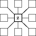
Let us start with a famous example which helped a lot to make the theory of CA almost popular: The "Game of Life" invented by J. H. Conway in 1970. It was his intention to investigate the evolution of an idealized population of living beings. It does not matter much that we cannot implement "Life" in a two-dimensional cellular space, as it was suggested by Conway; we will take a retina that is finite, though big enough instead. Furthermore we use two states 0 and 1: A cell will represent a living organism, if its state is 1, and a dead one, if the state is 0. The neighbourhood will include the cell z refered to (generic cell) itself, together with the eight surrounding cells.


2-dimensional Moore Neighbourhood

Fig. 3: Neighbourhood used for "Life".

The evolution of the population obeys the following rules:

Though these are very simple rules to model phenomenoms like the deadly consequences of a too high or too low population density, or the birth of new life under good conditions, the behaviour of such a system is already so complex that it could hardly be overseen. One reason for that surely is that the chosen rules are very balanced.


SIGMA life;

DIMENSION 2;

REGISTER INT state;

NEIGHBOUR  center       : ( 0, 0);
           left         : (-1, 0);
           right        : ( 1, 0);
           upper        : ( 0, 1);
           lower        : ( 0,-1);
           left_upper   : (-1, 1);
           right_upper  : ( 1, 1);
           left_lower   : (-1,-1);
           right_lower  : ( 1,-1);

VAR INT sum;

BORDER {0};


TABLE

   sum = center.state
	  + left.state + right.state + upper.state + lower.state 
	  + left_upper.state + right_upper.state
	  + left_lower.state + right_lower.state;

   sum==3; : SELF={1}; :

   sum==4; : /* no statement */ :

   /* TRUE */ : SELF={0}; :

The program given here can be recognized as a SDL program by the keyword SIGMA in the headline. It desribes what the local rule function will do to a single but arbitrary cell of the retina during one step of the simulation. The program consists of two parts: The first part reachs until TABLE and includes several declarations:

The second part shows the rules of evolution as kind of some (here: three) nested IF-THEN-ELSE statements (entries). Notice that all IF, THEN and ELSE parts are separated from each other by colons : . Everywhere in the table part, assignments to variables are allowed; Here, the total number of neighbours with state 1 is stored first in sum. Later sum is used to choose a proper action.
Observe that a non existent condition - like in entry three - equals TRUE and that the generic cell is left invariant, if there is no statement in the consequence part - like in entry two.


RETINA glider;

RANGE [0,0]..[10,10];

REGISTER INT state;

START
      [1,2]= {1};
      [2,3].state = 1;
      [3,1]..[3,3] = {1};
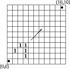
Glider


The RDL program shown above describes an initial configuration that matches the SDL program Life. Again we find a subdivision into a declaration and a statement part:

Applying the local rule Life to this initial configuration, the figure consisting of state-1-cells will appear again after five time steps, but shifted up and to the right one cell each.

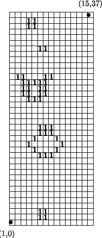
By the way, the following strange-looking initial configuration answered the question raised by Conway, if there exist populations whose size will approach infinity in time, assuming that there is enough space. (Hint: The solution is close connected with the first figure.)


RETINA strange;

RANGE [-10,-10]..[30,40];

REGISTER INT state;

START
      [6,1]..[7,2]       = {1};

      [6,12]..[8,12]     = {1};
      [5,13] (4) [9,13]  = {1};
      [4,14] (6) [10,14] = {1};
      [5,15] (4) [9,15]  = {1};
      [6,16]..[8,17]     = {1};

      [4,22]..[6,22]     = {1};
      [3,23]..[7,25]     = {1};
      [5,23]..[5,24]     = {0};
      [2,26] (6) [8,26]  = {1};
      [3,26] (4) [7,26]  = {1};

      [6,31]..[7,31]     = {1};

      [4,35]..[5,36]     = {1};
A glider cannon


Remark:
The device [5,15] (4) [9,15] = {1}; assigns 1 to a couple of cells within the rectangle [5,15] .. [9,15]: exactly to every fourth cells in each coordinate direction starting with the cell in [5,15].

Source Code: life.sdl
glider.rdl
cannon.rdl

previous contents index next
(CA in SCARLET..) Contents Index (..CA in SCARLET)