
(Introduction)	Contents	Index	(CA in SCARLET..)

1. Cellular Automata

1.1 Formal Definitions

In order to give readers who are not very acquainted to CA a chance to come to remarkable results in SCARLET after a short time, we are going to introduce CA by some basical definitions and to explain it with some examples before looking at SCARLET itself. Readers who are already used to CA this chapter may serve to make sure of the notation used here. Most of the definitions given here are taken from the report ''Parallele Automaten'' of Martin Kutrib[5].

We approach the definition of CA by examining the definition of cellular spaces first:

A 5-tuple

is called cellular space, if it holds:

S is a finite state set, which is not empty.
is the space dimension.
N is a n-tuple of pairwise different elements of , , called d-dimensional neighbourhood of order n.
is the local rule function
is the quiescent state, which suffices: .

Are you already in the mood to give up? We hope not, because although precise definitions are sometimes a bit abstract and difficult to see through, the idea of CA hidden somewhere between the lines, is amazingly concrete:

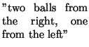
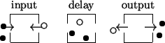
First of all we consider a single Moore-automaton, which has got

a finite and non-null state set S - exactly like the cellular space,
a mapping that calculates an output just depending on the state the automaton has got at that moment (output function),
a mapping that computes the state of the automaton in the next time step having the current state and an input as arguments (transition function).

(Furthermore Moore-automata have got initial and final state sets, too, but we will ignore that, since it does not play an important part in the following explanations.)

''Could you please repeat at which point exactly I should have got the idea of it???'' Really, did it not become clear? Whenever we speak of an automaton in daily life, we most of the time actually mean an object that can theoretically be described by a Moore-automaton!

You cannot believe that? Perhaps the following example will convince you:

Example 1: The "Input/Output Automaton"(IO-A)

Consider a little machine in a box with two holes, each of them on opposite sides, such that the machine can fulfil only one (boring) task: to eject balls that have been inserted on one side, one by one on the other side after a small delay, where no more balls will be accepted. The machine permits to use both holes as slots.

Now we are going to show that we can model the IO-A as a Moore-automaton. First of all we need a suitable state set. Observe that a state is, for example, conveniently specified by the number and origin of all balls within the automaton during the time of delay ("no ball"; "one ball from the right, two from the left", and so on). Like that the set of all possible states S is not empty, but finite for there can only be a finite amount of balls within the automaton at a time.
Further, states and outputs are related to each other in a unique way (the output function

exists and is bijective):

1.
2.

Fig. 1: Different possible states of an IO-A.

It is easy to comprehend that there exists the same relationship between the state set and the set of inputs; in particular we have the transition function

as postulated above. (In this simple example it isjust depending on the input, not on the current state.)

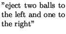
''Ok, ok; but what have Moore-automata to do with cellular spaces?'' That will be the next step; in fact a cellular space consists of an infinite number of automata of the same type, which are communicating with each other. - But let us return to our example:

Example 2: One-dimensional IO-A cellular space:

Assume now an infinite amount of IO-A lined up such that the slots of each two automata standing next to each other touch. Now their positions could be labeled with elements of

; in other terms: The IO-A are ordered in the one-dimensional space

Besides we consider all IO-A to be in the same rhythm of time, that means the periods of input, output, and delay happen for all of them to be at the same time.

By consequence of this construction, each automaton has got a left and a right neighbour, whose outputs will determine its input. Conversely its own output will influence the inputs of other IO-A.
Because of the fact that is bijective, we can identify the output of an IO-A with the state it has at that moment and could, therefore, say:

: The state of an IO-A in the next time step is completely determined by the current states of its neighbours.

(Since cellular spaces are always constructed of Moore-automata with bijective output function , it is not longer necessary to speak of input and output. It is convenient to care about the states instead.)

Fig. 2: Two timesteps in the evolution of an IO-A cellular space.

Arriving at that point we have already found a local rule function

that seems to be convincing: Starting from two states it computes a new state in such a way that this is the state of an IO-A, if the arguments have been the preceding states of its left and right neighbour. Hence the neighbourhood is of order two and the quiescent state q₀ finally is the state "no ball", for an I/O-A will not have a ball, if its neighbours have not had one in the previous time step.

''But who tells us we've chosen the right function ? The definition doesn't tell anything about that! Anyway, what about this strange n-tuple that is said to be the neighbourhood? It seems that it isn't useful at all, otherwise it would have been already mentioned?!''

Just a moment! These points are still unclear, because we have always emphazised that cellular spaces are accumulations of single automata with a high degree of independence. But in fact one focuses on the cellular space as a whole, with a homogeneous behaviour and regards the automata only as its components. (That is the reason why they are also called cells (or sites).) The following definitions allow the use of such a point of view that looks at a cellular space in its totality, and, therefore, complete our explanations:

A mapping

is called configuration of the cellular space at time step

. c₀ is also labeled initial configuration.
c_t(i),

, is called state of the automaton i under the configuration c_t.

Suppose that A denotes an alphabet, a d-dimensional neighbourhood, and C_d the set of all configurations . A mapping is called global mapping, if it is induced by a local rule function as follows:

For all is valid:

The most important tool to look at a cellular space as a whole seems to be the configuration: Each configuration presents the states of all automata at a certain time step. Consequently now we are looking for a (global) mapping that will convert in a suitable way whole configurations. We have found the right one, when its global actions can be reduced on the local effects of on every cell. - Obviously this is only possible, if the elements of the cellular space, the automata, are homogeneous!

Example 2 (Resumption):: If we choose the 2-tuple N=(-1,1) as the neighbourhood, we obtain for all and :

Taken in account that applied to the states of the left and right neighbour yields the state of the IO-A in i in the following time step, thus c_t+1(i) with c_t+1 the successor configuration of c_t will lead us to the conclusion that the global mapping exists. At the same time, the example should have helped to make the connection between , , and N a bit clearer.

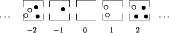
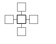
In the example given above, those cells that had an influence on the successor state of another cell were also its spatial neighbours. Because that is a general (though not necessary) phenomenom, one speaks just of "neighbours with regard to a certain neighbourhood", when those cells which are the arguments of the local rule function for a certain site, are meant, or in more formal terms:

Suppose that

is a cellular space. Let

. Then, a cell i is called neighbour of cell j with regard to N, if there exists a component k of N such that i = j+k.

In other words, the neighbourhood indicates the relative positions of an arbitrary cell to its neighbours.
In particular a cell may be its own neighbour, if N contains the component .

Example 3:

A quite common example of a d-dimensional neighbourhood is the so-called ''general von Neumann neighbourhood''

$H^d_k:={i in ZZ^d: sum_{n=1}^d{i_n}<= k}$

For d = 2 and k = 1 we obtain the following structure:

H₁²:

Unlike the Moore-automata mentioned in the beginning, the main purpose of cellular spaces is not the construction of real existing machines, as well as software, which is e.g., capable of pattern recognition and so on, but the discrete simulation of continuous systems, as known, for instance, from the natural sciences, for both a better comprehension of the theory of dynamical systems, and practical calculations.
Therefore, not seldom cells are intended to model discrete points of a system in ; states contain discrete physical quantities or they just tell, if there is a particle located in that point; and the local rule is meant to imitate some laws of nature.

Because all real existing systems are subject to certain material restrictions - probably this is less obvious for real systems than for simulation systems - we are usually more interested in a finite form of cellular spaces: the cellular automaton (CA).

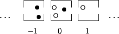
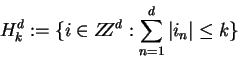
Suppose that

is a cellular space. M is called cellular automaton if the following is true:

There exists such that for all and for all :

$c_{t+1}(i)=# <=> c_t(i)=#$

# is called boundary value.
Suppose
B := { : There exists , such that l is a neighbour of i }.
A finite, not empty domain , called retina (or lattice) has the following properties:
- For all :
- For all :
- For all : c₀(k) = q₀
- For all : i is neighbour of j with regard to the v. Neumann neighbourhood H₁^d - directly or with mediator neighbours in between - or the other way around.

In contrast to cellular spaces the area of interest of a CA lies within a fixed subset of , the so-called retina. The last condition of 2., which demands that the cells are organized in undisrupted lines along the coordinate axes, guarantees that the set is a connected domain.

It is bounded by the set B, that means that B contains all cells which are neighbours of cells within the range of the retina, but which are not lying in the interior themselves. Therefore, B is called boundary or border. All cells on the boundary - and only those - remain in a particular state # all the time; so their influence on the retina is always the same.
Furthermore those cells lying behind the boundary are - because of the definition of B - neighbours to no cell in retina and, therefore, do not have any influence on it.
If we are only interested in the behaviour of a cellular space within a certain area, we do not need to hesitate to forget the world behind the boundary. We could assume, for instance, that all cells there have got the quiescent state at t = 0.


(Introduction)	Contents	Index	(CA in SCARLET..)